Lei Feng: According to Gao Xiang, a doctoral student at the School of Automation , Tsinghua University, the main research interest is visual SLAM technology based on RGB-D cameras. He has received Tsinghua Freshman Scholarship, Zhang Mingwei Scholarship and won the national inspirational scholarship three times. The relevant research results were published in journals and conferences such as Robotics and Autonomous Systems, Autonomous Robot, CCC, and personal blogs (click to view) . The original title is: "The robot's eyes: Visual SLAM Introduction."
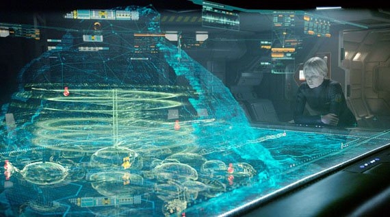
It has been nearly three years since SLAM (Simultaneous Robot Positioning and Mapping) began to be studied. From the first year of Ph.D., he became interested in this direction. Up till now, he has been given a general understanding of this field. However, the more you understand, the more you think this direction is difficult. In general there are several reasons:
1. Little information on getting started. Although there are many people in the country who are still doing it, there is not a good introduction to it. SLAM for dummies can be considered an article. There is almost no Chinese material.
2. SLAM research has been going on for more than 30 years, starting in the 1990s. There are also a number of historical branches and disputes. It takes a lot of work to grasp its direction.
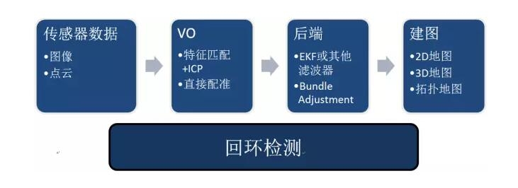
3. It is difficult to achieve. SLAM is a complete system composed of many branch modules. Now the classic program is a trilogy of "image front-end, optimized back-end, closed-loop detection", and many documents cannot be realized by themselves.
4. Do-it-yourself programming requires a lot of pre-requisite knowledge. First you need C and C++. A lot of code on the Internet also uses 11 standard C++. The second will use Linux. The third will be cmake, vim/emacs and some programming tools. The fourth will use openCV, PCL, Eigen and other third-party libraries. Only after learning these things can you really start to compile a SLAM system. If you want to run an actual robot, you will also need ROS.
Of course, more difficulties means more gains, and bumpy roads can exercise people (for example, walking and finding that Linux and C++ are my true love.) Given that there is currently very little information on visual SLAM on the Internet, I So I wanted to share my experience with this three years. Whatever is wrong, please criticize and correct me.
This article focuses on visual SLAM, which refers specifically to the use of cameras, Kinect, and other depth cameras for navigation and exploration. It focuses on interior parts. So far, the framework of visual SLAM has been basically mature, and it can be positioned and constructed within a centimeter-level error range in a stable and well-lit environment. However, there is still a long way to go to apply visual SLAM technology away from a dynamic environment filled with dynamic lighting and crowds. Below, I will introduce the history, theory, and implementation of SLAM, and introduce the implementation of visual (Kinect).
| SLAM issues SLAM, the full name is Simultaneous Localization and Mapping, Chinese is called simultaneous positioning and mapping. In general, a SLAM system is divided into four modules (removing sensor data reads), as shown in the following figure:
Ah no, so to speak, this article is definitely no one to read, so we change one way to introduce the robot "small radish" classmates.
The story of radish
In the past, there was a robot called "radish." It has a pair of big black eyes, called Kinect. One day, it was slammed into an empty room by evil scientists. It was filled with miscellaneous things.
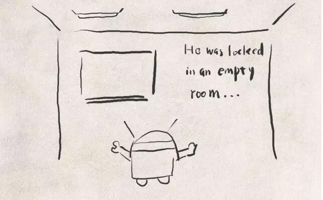
The radish was terrified because he had never been to this place and did not understand it at all. There are three main issues that make him feel scared:
1. Where are you?
2. What is this place?
3. How to leave this place?
In SLAM theory, the first problem is called Localization, the second is called Mapping, and the third is subsequent path planning. We hope to use the Kinect tool to help radish solve this problem. What ideas do students have?
| Kinect dataTo defeat the enemy, you must first understand your weapon. Well, let's introduce Kinect first. It is well known that this is a depth camera. You may have heard of other brands. However, the price of Kinect is low, the measurement range is between 3m-12m, and the accuracy is about 3cm. It is more suitable for indoor robots such as radish. The image it picks up is like this (rgb map, depth map and point cloud map from left to right):

One of Kinect's strengths lies in the relatively low cost of obtaining each pixel's depth value, both in terms of time and economics. OK, with this information, radishes can actually know the 3d position of each point in the picture it captures. As long as we calibrate the Kinect in advance, or use the factory calibration.
We set the coordinate system to this, which is the default coordinate system used in openCV.
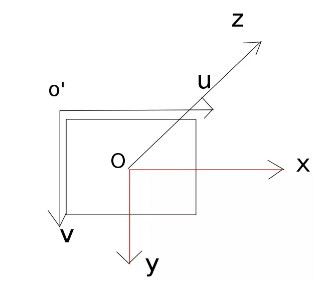
O'-uv is the image coordinate system and o-xyz is the coordinate system of Kinect. Suppose the point in the picture is (u, v) and the corresponding 3D point position is (x, y, z), then the conversion relationship between them is as follows:

Or more simple:
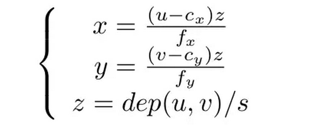
The latter formula gives the method for calculating 3D points. First read the depth data from the depth map (Kinect gives a 16-bit unsigned integer) and remove the z-direction scaling factor so that you change an integer to data in meters. Then, x, y is calculated using the above formula. It is not difficult at all, it is a center point position and a focal length. f represents the focal length and c represents the center. If you do not calibrate your Kinect yourself, you can also use the default values: s=5000, cx = 320, cy=240, fx=fy=525. The actual value will have a slight deviation, but not too much.
| Location issuesOnce we know the position of each point in the Kinect, what we need to do next is to calculate the displacement of the radish based on the difference between the two images. For example, the following two figures, the latter one is collected in 1 second after the previous one:
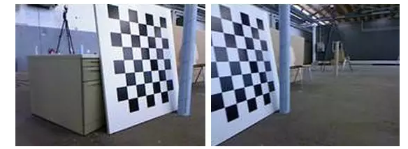
You can certainly see that the turnip turned right to a certain angle. But how much has it turned? This depends on the computer to solve it. This problem is called camera relative pose estimation. The classic algorithm is ICP (Iterative Closest Point).
This algorithm requires knowledge of a set of matching points between the two images. The popular point is that the left image is the same as the right one . Of course you see that black and white board appears in both images.
In the view of radish, two simple problems are involved here: the extraction and matching of feature points.
If you are familiar with computer vision, you should have heard of features like SIFT, SURF. Well, to solve the positioning problem, we must first get a match between two images. The basis of matching is the characteristics of the image. The following figure shows the key points and matching results extracted by SIFT:
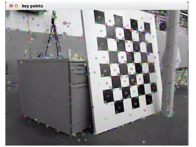
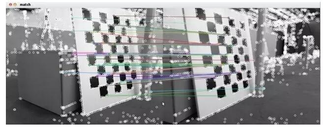
Students who are interested in implementing code can use Google's "opencv match" method. There are also clear examples of openCV tutorials. The above example shows that we found some matches, but some of them are correct (basically equal match lines) and some are wrong. This is because there are periodic textures (black and white blocks) in the image, so it is easy to make mistakes. But this is not a problem. We will eliminate these effects in the next steps.
After we get a set of matching points, we can calculate the conversion relationship between the two images, also called the PnP problem. Its model is this:
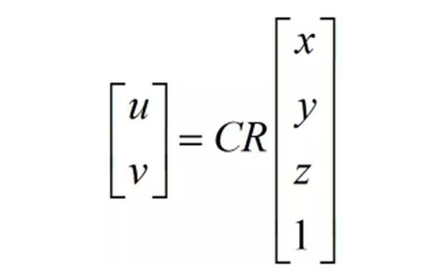
R is the attitude of the camera and C is the calibration matrix of the camera. R is constantly moving, and C is dead with the camera. The ICP model is slightly different, but in principle it is also the calculation of the camera's attitude matrix. In principle, this matrix can be counted as long as there are four sets of matching points. You can call OpenCV's SolvePnPRANSAC function or PCL's ICP algorithm to solve. The algorithm provided by openCV is a RANSAC (Random Sample Consensus) architecture that eliminates false matches. So when the code actually runs, it can find the matching point. The following is an example of a result.
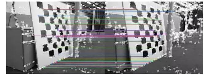
The two figures above turned 16.63 degrees, with almost no displacement.
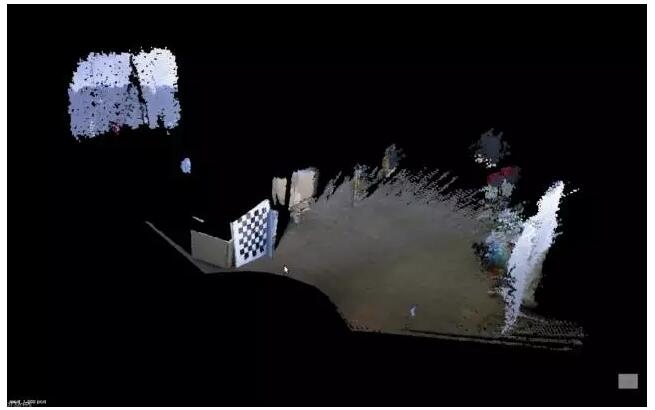
Some students will say, as long as it continues to match, positioning problem is not resolved? On the surface, this is indeed the case, as long as we introduce a keyframe structure (defined as a keyframe when the displacement exceeds a fixed value). Then compare the new image with the keyframe. As for the construction of the map, it is to put together the key cloud of these key frames, watching there is a pattern, like:
However, if things are so simple, the SLAM theory will not have to be studied by so many people for more than thirty years (it was studied since the 1990s). (Those above mentioned things can be done simply by finding a small master degree. ......). So where is the problem difficult?
| SLAM end optimization theoryThe most troublesome issue is "noise." This asymptotic matching method, like those of inertial measurement equipment, has accumulated noise. Because we are constantly updating keyframes, we compare the new image with the nearest keyframe to obtain the robot's displacement information. But you have to think that if there is a shift in one of the keyframes, then the remaining displacement estimate will have one more error. This error will also accumulate because the following estimates are based on the previous robot position...
Wow! This result is simply unbearable. For example, your robot turns 30 degrees to the right and 30 degrees to the left to return to its original position. However, due to errors, you are turning 29 degrees to the right and 31 degrees to the left, so that in the map you build, there will be two "ghosts" in the initial position.
Can we think of ways to eliminate this damn error?
Friends , this is SLAM's research. The front can be said to be the "image front-end" approach . Our solution is:
If you compare with the most recent keyframe, it will cause a cumulative error. Well, we'd better compare it to the earlier keyframes and compare a few more frames, not just one.
We use mathematics to describe this problem. Assume:
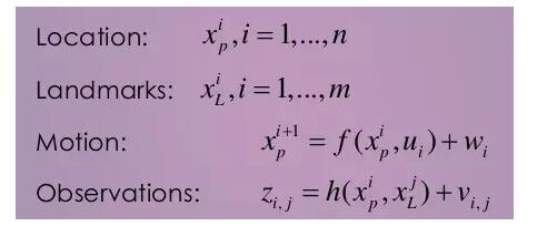
Do not be afraid. Only with mathematics can you clarify this issue. In the above formula, xp is the position of the robot radish, and we assume that it consists of n frames. xL is a roadmap. In our image processing process, we refer to the key points raised by SIFT. If you do 2D SLAM, then the robot position is x, y plus a corner theta. If it is 3D SLAM, it is x, y, z plus a quaternion gesture (or rpy gesture). This process is called parameterization.
No matter which parameter you use, you need to know the latter two equations. The former is called the equation of motion and describes how the robot moves . u is the input of the robot and w is the noise. The simplest form of this equation is how you can get the displacement difference between the two frames by means of a code wheel, etc. Then, this equation is directly added to the previous frame and u. In addition, you can also completely eliminate inertial measurement equipment, so that we only rely on image equipment to estimate, which is also possible.
The latter equation is called the observation equation and describes how those road signs come from. You saw the jth roadmap in the i-th frame and produced a measured value, which is the horizontal and vertical coordinates in the image. The last item is noise. Telling you secretly, this equation is exactly the same as the one on the previous page.
Before solving the SLAM problem, we need to see what data we have? In the above model, we know the motion information u and the observation z. This is schematically shown as:
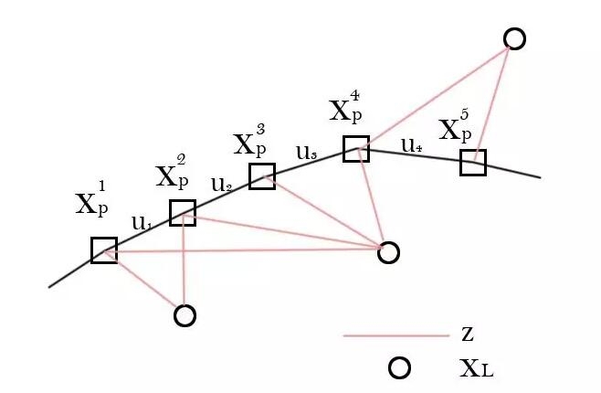
What we need to solve is to determine all xp and xL based on these u and z. This is the theory of the SLAM problem.
Scientists have been solving this problem since the birth of SLAM. Initially, we used a Kalman filter , so the above model (motion equation and observation equation) was built like this. Until the beginning of the 21st century, the Kalman filter still occupied the most important position in the SLAM system. Davison's classic monocular SLAM was made with EKF. But later, SLAM method based on graph optimization emerged, gradually taking its place [1]. We don't introduce the Kalman filter here. Interested students can find the Kalman filter on the wiki. Another Chinese introduction to the Kalman filter is also great. Because the filter method stores n landmarks and consumes n squared space, it is a bit unbalanced by the amount of computation. Although it was proposed in 2008 that the filters of the divide-and-conquer method could bring the complexity to O(n) [2], the means of realization are more complicated. We want to introduce the emerging method: Graph-based SLAM .
The graph optimization method makes the SLAM problem an optimization problem. Students who have studied operations research should understand how important optimization issues are to us. Are we not asking for the robot's position and signpost position? We can make a guess first and guess where they are probably. This is actually not difficult. Then, the error can be calculated by comparing the guess value with the value given by the motion model/observation model:
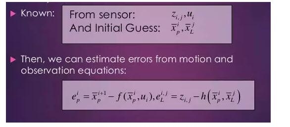
In a nutshell, for example, I guess the first frame of the robot is at (0,0,0) and the second frame is at (0,0,1). However, u1 told me that the robot walked 0.9 meters in the z direction (forward), then the equation of motion showed an error of 0.1m. At the same time, in the first frame, the robot found the landmark 1 and it was in the middle of the robot image; the second frame found it in the middle right position. At this time we guessed that the robot just went forward and there was an error. As for this error, it can be calculated from the observation equation.
We get a bunch of errors, add these squared errors together (because the simple error has positive and negative, but the square error can be changed to other norms, but the square is more commonly used), and the sum of squared errors is obtained. Let us call this phi the objective function of our optimization problem. The optimization variables are those xp, xL.

To change the optimization variable, the sum of squared error (objective function) will become larger or smaller accordingly. We can use numerical methods to find their gradient and two-step gradient matrix, and then use the gradient descent method to find the optimal value. Those who have learned to optimize things understand.

Note that there are often thousands of frames in a robot SLAM process. Each frame we have hundreds of key points, one multiplication is millions of optimization variables. This scale of optimization issues into the small radish on the air can be solved? Yes, past classmates thought that Graph-based SLAM cannot be calculated. However, some students found out after the years of 06 and 07 in the 21st century that the scale of the problem was not as large as it was imagined. The above two J and H matrices are "sparse matrices," so we can use sparse algebra to solve this problem. The reason for “sparseness†is that each road sign is often impossible to appear in all movements, usually only in a small part of the image. It is this sparseness that makes optimization ideas a reality.
The optimization method makes use of all available information (called full-SLAM, global SLAM), and its accuracy is much higher than the inter-frame matching we started with. Of course, the amount of calculation is also higher.
Due to the sparsity of optimization, people like to use "graphs" to express this problem. The so-called graph is composed of nodes and edges. I wrote G={V,E} and everyone understood. V is the node of the optimization variable and E represents the constraint of the motion/observation equation. What is more confused? Then I will take a picture from [3].
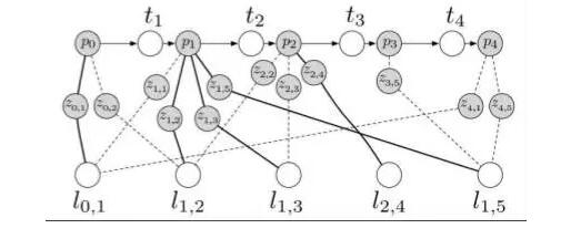
The figure is a little blurry, and the math symbols are not quite the same as the ones I use. I use it to give you an intuitive image of graph optimization.
In the figure above, p is the robot position, l is the road sign, z is the observation, and t is the displacement. Among them, p, l are optimization variables, and z, t are optimization constraints. Does it look like some springs connect some particles? Because each landmark is unlikely to appear in every frame, this graph is sparse.
However, "graph" optimization is only an expression of the optimization problem and does not affect the meaning of optimization . The actual solution is still to use numerical methods to find the gradient. This idea is also called Bundle Adjustment in computer vision. Its specific method, please refer to a classic article [4].
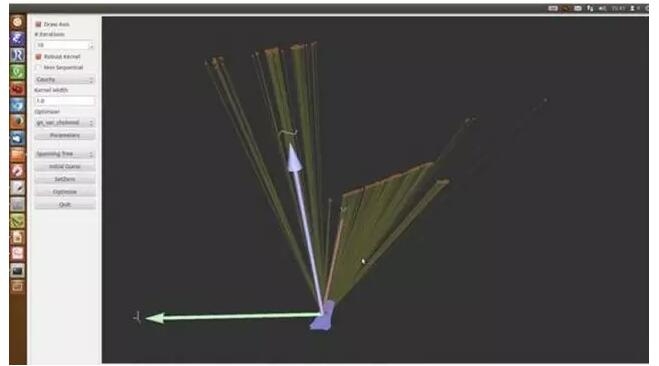
However, the implementation of BA is too complicated and it is not recommended that students use C to write. Fortunately, on the 2010 ICRA, other students provided a generic development kit: g2o [5]. It is a general-purpose solver with map optimization. It is very useful. I will introduce this package in detail in the next day. In short, we just throw observations and motion information into the solver. This optimizer will find the robot's trajectory and landmark position for us. As shown below, the red dot is a road sign and the blue arrow is the robot's position and corner (2D SLAM). Attentive classmates will find it deflecting a little to the right:
As mentioned above, the problem of using only the largest frame-to-frame matching is the accumulation of errors. The graph optimization method can effectively reduce the accumulated error. However, if all the measurements are dropped into g2o, the amount of calculation is still a bit large. According to my own test, about 10,000 sides, g2o is a bit difficult to run. In this way, some students said that they can concisely construct the map. We don't need all the information. We only need to get useful information out.
In fact, when radishes are exploring the room, they often turn left and turn right. If at some point he returned to where he had been before, we would compare directly with the keyframes collected at that time, could that be? We say, yes, and that's the best way. This problem is called closed-loop detection.
Closed-loop detection means that when you come to an image, how do you tell if it has previously appeared in the image sequence?
There are two ways to think about it: first, to see if it is close to a previous location based on our estimated robot position; and second, to see if it is similar to the previous keyframe based on the appearance of the image.
At present, the mainstream method is the latter, because many scientists believe that the former relies on noise to reduce the noise position, a bit of circular argument. The latter method, in essence, is a pattern recognition problem (unsupervised clustering, classification), commonly used is Bag-of-Words (BOW). However, BOW needs to train the dictionary in advance, so SLAM researchers are still exploring whether there is a more appropriate method.
In Kinect SLAM's classic masterpiece [6], the authors used a relatively simple closed-loop approach: k randomly selected from the first n keyframes, and matched each other with the current frame. After matching, think that there is a closed loop. This is really quite simple and practical, and efficiency is decent.
Efficient closed-loop detection is the basis for the exact solution of SLAM. Researchers are also trying to use deep learning techniques to improve the accuracy of closed-loop detection. For example, the author of this article published in the Journal of Autonomous Robot Unsupervised Learning to Detect Loops Using Deep Neural Networks for Visual SLAM System uses an unsupervised deep automatic encoder from the original The learning of a compact image representation in the input image improves the robustness of the closed-loop detection compared to the traditional Bag of Word method. The method flow chart is as follows [7]:

In this paper, we introduce the basic concepts of SLAM and focus on the idea of ​​graph optimization to solve SLAM problems. The author of this article has written a SLAM program based on RGB-D camera (click to enter the github address), which is a cmake-based project under Linux.
references
[1] Visual SLAM: Why filter? Strasdat et. al., Image and Vision Computing, 2012.
[2] Divide and Conquer: EKF SLAM in O(n), Paz Lina M et al., IEEE Transaction on Robotics, 2008
[3] Relative bundle adjustment, Sibley, Gabe, 2009
[4] Bundle adjustment - a Modern Synthesis. Triggs B et. el., Springer, 2000
[5] g2o: A General Framework for Graph Optimization, Kummerle Rainer, et. al., ICRA, 2011
[6] 3-D Mapping with an RGB-D Camera, IEEE Transaction on Robotics, Endres et al., 2014
[7] Xiang Gao, Tao Zhang, Unsupervised Learning to Detect Loops Using Deep Neural Networks for Visual SLAM System, Autonomous Robot, 2015.
Lei Feng Network (search "Lei Feng Network" public number attention) Note: This article was published by the author in the deep learning lecture, reproduced please contact the authorize and retain the source and author, not to delete the content.